1.1 Logic and Proofs (part 1)

First, we are going to start with logic because it is a branch of mathematics and philosophy concerned with reasoning and argumentation which means that based on this reasoning we have practically working applications in our computers be it the correctness of computer programs, ensuring the quality and reliability of software systems, prove the security of cryptographic algorithms and many many more.
So, we have our reasoning in place the only thing which is left now is to validate our reasoning and for that, we need something called Proof.
Proofs, in mathematical logic, are a series of logically deduced statements used to establish the truth of a proposition or theorem (once we prove a mathematical statement is true, we call it a theorem) and the concept of a proof is used to demonstrate the correctness of algorithms and to establish the validity of logical systems.
The examples for both of them combined are in the vast array be it optimizing schedules, finding the shortest path between two points, determining the most efficient way to use resources, choosing between different options, evaluating risks and benefits, and weighing trade-offs.

Starting from the very first thing in logic is a statement, also called a proposition, which will be declarative in its nature. That is it can be either true or false. In propositional logic, we use symbols to represent propositions, and logical connectives (such as "and", "or", "not", "implies", etc.) to build complex expressions.

Examples of valid propositions-

• New Delhi is the capital of the Indian Republic.
• 1+1 = 2 (There is a 300-page book Principia Mathematica for this)
• Jang (my friend) was born in Manipur.

Examples of invalid propositions-

• Do this!
• Stand-up!
• What a beautiful day!
• Is the sun hot?

Two things are here- FIRST since in mathematics we usually deal with problems(statements) in the form of variables to avoid writing those lengthy statements and we are going to use p, q, r, s, . . . as the variables to represent the individual statements. It's not compulsory but is somewhat like a standard which is followed by people and even in programming we tend to use i, j, k, . . . as the inner variable in loops.

SECOND is to create new propositions which are statements constructed by combining one or more propositions. You can think of this in a way for example your friend said to you that he talked to this very girl/boy and your response to that information highly probably is no way you talked to her/him.

Let's try to represent this in the above-discussed paras -

let p be the statement said by your friend

p = I talked to this girl/boy.

let q be the statement which you said to your friend

q = You can't talk to that girl/boy.

Do you see any inference from here?

The thing which I wanna convey from here is that the very thing which you usually do with your friend is to oppose what they'd said just to tease them. But, what it actually does is this starts to build your conversation between you and your friend i.e. makes your conversation complex and fun.

This is exactly what we do here once we have our statements in place we try to make them more complex so that we can optimise and better solution in the end.

Let p be a proposition. The negation of p, denoted by ¬p

p : Jang is a good PC gamer.

¬p : Jang is not a good PC gamer.

Now, we've done converting the statements into the variables and somewhere started making statements more complex by combining more statements together.

We are now at the point of combining both of them into the tables which are known as a truth table.

A truth table is a table used in logic and mathematics to evaluate the truth value of a proposition or an argument. A truth table lists all possible combinations of truth values for the propositions involved and shows the resulting truth value of the whole statement.

A truth table has one row for each possible combination of truth values of the propositions, and the columns represent the propositions involved in the statement. The last column of the truth table contains the true value of the whole statement, based on the truth values of the propositions.

Here, is the Truth table for the Negation of a proposition

  

p	¬p
T	F
F	T

Now, if you pay a little attention to your own language there are always some connectivities so that you can create more complex propositions.

Such basic two are also available here and they are and & or.

They are represented by ∧ & ∨(also known as conjunction & disjunction)

In the English language connectivity or is taken in two ways what I mean is sometimes when it's used it can also include both sentences i.e inclusive or sometimes it refers that only one sentence out of the connected two sentences can be valid not both at the same time i.e. excluding.

So, the inclusive or is represented with the same symbol above but to make a distinction for the exclusive or we use the symbol ⊕

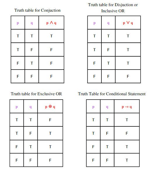
Now, we have seen conjunction, disjunction and Xor it's time to see -

Conditional statements are nothing but if p then q which means the first thing only happens when the sufficient condition of the next dependent statement occurs and this is represented as p → q.

There are some variations to the same -

“if p, then q” “p implies q” “if p, q”

“p only if q” “p is sufficient for q”

“a sufficient condition for q is p” “q if p”

Here's an example of a conditional statement:

"If it rains, then I will carry an umbrella."

In this example, the event is "it rains" and the consequent is "I will carry an umbrella." If it rains, then the event is true and the whole statement is true. If it doesn't rain, then the event is false and the whole statement is true.

There are three more things which are related to this Converse, Contrapositive and Inverse. Let's look at them -

The proposition q → p is called the converse of p → q.

The contrapositive of p → q is the proposition ¬q → ¬p.

The proposition ¬p → ¬q is called the inverse of p → q

Here's an example to illustrate the concepts of converse, contrapositive, and inverse:

"If it is raining, then the streets are wet."

• Converse: "If the streets are wet, then it is raining."
• Contrapositive: "If the streets are not wet, then it is not raining."
• Inverse: "If it is not raining, then the streets are not wet."

There is something also called a biconditional statement and it's represented by p ↔ q. It's true when both p & q have the same truth values.

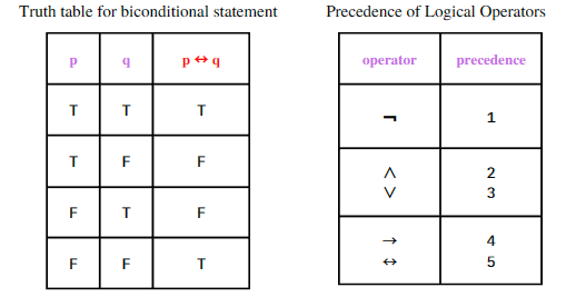
Predicates and Quantifiers are fundamental concepts in mathematical logic.

A predicate is a function that maps elements of a set to truth values (true or false).

Predicates can be used to describe the properties of elements in a set. For example, the predicate "x is an even number" can be applied to elements of the set of integers to determine whether they are even or odd.

Quantifiers are symbols used to express the number of elements in a set that satisfy a predicate. The two most common quantifiers are the universal quantifier (∀) and the existential quantifier (∃).

• The universal quantifier (∀) expresses that a predicate is true for all elements in a set. For example, "for all x in the set of natural numbers, x > 0" can be expressed as ∀x (x > 0).
• The existential quantifier (∃) expresses that there exists at least one element in a set that satisfies a predicate. For example, "there exists a natural number x such that x > 10" can be expressed as ∃x (x > 10).

Rules of inference

why rules of inference are needed in logic and proofs?

Rules of inference are needed in logic and proofs because they provide a systematic method for deducing new conclusions from given premises. These rules are based on logical relationships between propositions, and they allow us to determine whether a conclusion logically follows from the premises.

By using rules of inference, we can build logical arguments that are valid and can be used to prove theorems, solve problems, and make decisions.

Here, is the video for the same.

Awesome way to learn from YouTube

 Me Devansh after many years finally started doing what I always wanted to do and that is to share my knowledge in a way how I learn and understand things.

Link to the channel - Kyuantym

My first video

In this channel I am basically explaining my learnings.

How to do Object Detection with OpenCV | Tutorial

Disk Scheduling Algorithms

Disk Scheduling Algorithms

This tutorial is prepared for those that need assistance in Disk Scheduling Algorithms.

INTRODUCTION

In operating systems, seek time is very important. Since all device requests are linked in queues, the seek time is increased causing the system to slow down. Disk Scheduling Algorithms are used to reduce the total seek time of any request.

PURPOSE
The purpose of this material is to provide one with help on disk scheduling algorithms. Hopefully with this, one will be able to get a stronger grasp of what disk scheduling algorithms do.



There are many Disk Scheduling Algorithms but before discussing them let’s have a quick look at some of the important terms:
Seek Time:Seek time is the time taken to locate the disk arm to a specified track where the data is to be read or write. So the disk scheduling algorithm that gives minimum average seek time is better. 
Rotational Latency: Rotational Latency is the time taken by the desired sector of disk to rotate into a position so that it can access the read/write heads. So the disk scheduling algorithm that gives minimum rotational latency is better.
Transfer Time: Transfer time is the time to transfer the data. It depends on the rotating speed of the disk and number of bytes to be transferred.
Disk Access Time: 
Disk Access Time = Seek Time + Rotational Latency + Transfer Time
TYPES OF DISK SCHEDULING ALGORITHMS
Although there are other algorithms that reduce the seek time of all requests, I will only concentrate on the following disk scheduling algorithms:

• First Come-First Serve (FCFS)
• Shortest Seek Time First (SSTF)
• Elevator (SCAN) 
• Circular SCAN (C-SCAN)
• LOOK
• C-LOOK 

These algorithms are not hard to understand, but they can confuse someone because they are so similar. What we are striving for by using these algorithms is keeping Head Movements (# tracks) to the least amount as possible. The less the head has to move the faster the seek time will be. I will show you and explain to you why C-LOOK is the best algorithm to use in trying to establish less seek time.
Given the following queue -- 95, 180, 34, 119, 11, 123, 62, 64 with the Read-write head initially at the track 50 and the tail track being at 199 let us now discuss the different algorithms.

1. First Come -First Serve (FCFS)
 
All incoming requests are placed at the end of the queue. Whatever number that is next in the queue will be the next number served. Using this algorithm doesn't provide the best results. To determine the number of head movements you would simply find the number of tracks it took to move from one request to the next. For this case it went from 50 to 95 to 180 and so on. From 50 to 95 it moved 45 tracks. If you tally up the total number of tracks you will find how many tracks it had to go through before finishing the entire request. In this example, it had a total head movement of 640 tracks. The disadvantage of this algorithm is noted by the oscillation from track 50 to track 180 and then back to track 11 to 123 then to 64. As you will soon see, this is the worse algorithm that one can use.

Advantages:

• Every request gets a fair chance
• No indefinite postponement

Disadvantages:

• Does not try to optimize seek time
• May not provide the best possible service

2. Shortest Seek Time First (SSTF) 
In this case request is serviced according to next shortest distance. Starting at 50, the next shortest distance would be 62 instead of 34 since it is only 12 tracks away from 62 and 16 tracks away from 34. The process would continue until all the process are taken care of. For example the next case would be to move from 62 to 64 instead of 34 since there are only 2 tracks between them and not 18 if it were to go the other way. Although this seems to be a better service being that it moved a total of 236 tracks, this is not an optimal one. There is a great chance that starvation would take place. The reason for this is if there were a lot of requests close to each other the other requests will never be handled since the distance will always be greater.

Advantages:

• Average Response Time decreases
• Throughput increases

Disadvantages:

• Overhead to calculate seek time in advance
• Can cause Starvation for a request if it has higher seek time as compared to incoming requests
• High variance of response time as SSTF favours only some requests

3. Elevator (SCAN) 
This approach works like an elevator does. It scans down towards the nearest end and then when it hits the bottom it scans up servicing the requests that it didn't get going down. If a request comes in after it has been scanned it will not be serviced until the process comes back down or moves back up. This process moved a total of 230 tracks. Once again this is more optimal than the previous algorithm, but it is not the best.

Advantages:

• High throughput
• Low variance of response time
• Average response time

Disadvantages:

• Long waiting time for requests for locations just visited by disk arm.

4. Circular Scan (C-SCAN) 
Circular scanning works just like the elevator to some extent. It begins its scan toward the nearest end and works it way all the way to the end of the system. Once it hits the bottom or top it jumps to the other end and moves in the same direction. Keep in mind that the huge jump doesn't count as a head movement. The total head movement for this algorithm is only 187 track, but still this isn't the mose sufficient.
5. C-LOOK 
This is just an enhanced version of C-SCAN. In this the scanning doesn't go past the last request in the direction that it is moving. It too jumps to the other end but not all the way to the end. Just to the furthest request. C-SCAN had a total movement of 187 but this scan (C-LOOK) reduced it down to 157 tracks.

From this you were able to see a scan change from 644 total head movements to just 157. You should now have an understanding as to why your operating system truly relies on the type of algorithm it needs when it is dealing with multiple processes.

NOTE: It is important that you draw out the sequence when handling algorithms like this one. One would have a hard time trying to determine which algorithm is best by just reading the definition. There is a good chance that without the drawings there could be miscalculations.

Programs related to these Algorithms -

/*
   Implementation of DISK Scheduling Algorithm using FCFS.
   Data structure used - ARRAY.
   Implemented by -  Devansh Varshney
   
   GitHub ID      -  varshneydevansh 
*/
#include<iostream>
#include<math.h>                                                             // For abs()
using namespace std;
int main(void)
{  
   int chart[100],result[100];                                               //Data Structure used
   int head,i,n,sum=0;
   cout<<"\n\tEnter the number of processes \n\t";
   cin>>n;
   cout<<"\n\tEnter the processes number \n\t";
   for(i=0;i<n;i++)
    {cin>>chart[i]; cout<<"\t";}                                            //Gettin' processes in the chart
   cout<<"\n\tEnter the HEAD number \n\t";
   cin>>head;
   for(i=0;i<n;i++)
   {
     result[i]=abs(chart[i]-head);
     head=chart[i];
   }
   
   for(i=0;i<n;i++)
   {
     sum+=result[i];
   }
   cout<<endl;
   for(i=0;i<n;i++)
   {
     cout<<"\t"<<result[i];
   }
   
  cout<<"\n\tSUM IS:\t"<<sum<<endl;
  return 0;

} //main()

//End of FCFS Algorithm

Polynomial Addition C-program w/ Output

Compiled and runned on Visual Studio Express 2013 for Windows Desktop

#define _CRT_SECURE_NO_WARNINGS

#include<stdio.h>

#include<stdlib.h>

#include<malloc.h>

struct polynode{

float coeff;

int exp;

struct polynode* link;

};

void create_poly(struct polynode** q) //Call by reference to provide address to original pointer

{

float c;

int e, flag;

struct polynode* temp = (struct polynode*) malloc(sizeof(struct polynode));

do{

if (*q == NULL)

{

*q = (struct polynode*) malloc(sizeof(struct polynode));

temp = *q;

}

else{

temp->link = (struct polynode*)malloc(sizeof(struct polynode));

temp = temp->link;

}

printf("\n\tEnter Coeffecient\n\t");

scanf("%f", &c);

temp->coeff = c;

printf("\n\tEnter Exponent\n\t");

scanf("%d", &e);

temp->exp = e;

 printf("\n\tWanna continue Y=1/N=0\n\t");

 scanf("%d", &flag);

} while (flag);

temp->link = NULL;

}

void display(struct polynode *q)

{

if (q==NULL)

{

printf("\n\tNot Found ! Try Again!!!\n\t");

return;

}

while (q != NULL)

{

printf("%fx^%d : ", q->coeff, q->exp);

q = q->link;

}

printf("\b\b\b");// Delete : from last

printf("\n\t");

}

void addpoly(struct polynode* p, struct polynode* q, struct polynode **r)

{

struct polynode *t = (struct polynode*) malloc(sizeof(struct polynode));// Temperary node

if (p==NULL && q==NULL)

{

return;

}

while (p != NULL && q != NULL)

{

if (*r==NULL) //Checking Total node where addition takes place

{

*r = (struct polynode*) malloc(sizeof(struct polynode));

t = *r; //Assigning temp to total node

}

else{

t->link = (struct polynode*) malloc(sizeof(struct polynode));// Creation of nodes at Intermediate Stage

t = t->link;

}

if (p->exp < q->exp)// If expo. of Second is greater then First assigining Second to Total

{

t->coeff = q->coeff;

t->exp = q->exp;

q = q->link;

}

else{

if (p->exp > q->exp)

{

t->coeff = p->coeff;

t->exp = p->exp;

p = p->link;

}

else{

if (p->exp == q->exp)

{

t->coeff = p->coeff+q->coeff;

t->exp = p->exp;

p = p->link;

q = q->link;

}

}//else

}//else

}//while-1

while (p != NULL)//If second list becomes empty or empty

{

if (*r == NULL) //Checking Total node where addition takes place

{

*r = malloc(sizeof(struct polynode));

t = *r; //Assigning temp to total node

}

else{

t->link = malloc(sizeof(struct polynode));// Creation of nodes at Intermediate Stage

t = t->link;

}

t->coeff = p->coeff;

t->exp = p->exp;

p = p->link;

}//while-2

while (q != NULL)//If first list becomes empty or empty

{

if (*r == NULL) //Checking Total node where addition takes place

{

*r = malloc(sizeof(struct polynode));

t = *r; //Assigning temp to total node

}

else{

t->link = malloc(sizeof(struct polynode));// Creation of nodes at Intermediate Stage

t = t->link;

}

t->coeff = q->coeff;

t->exp = q->exp;

q = q->link;

}//while-3

t->link = NULL;  //At last Make total NULL

}//polyadd()

void main()

{

struct polynode *first, *second, *total;

first = second = total = NULL;

int ch;

while(1)

{   

printf("\n\t Enter choice \t 1. First Expression\t2. Second Expression\t3.Addition\t4.exit\n\t");

scanf("%d", &ch);

switch (ch)

{

case 1:printf("\n\tCreate 1st expression\n\t");

create_poly(&first);

printf("\n\tStored the 1st expression\n\t");

display(first);

break;

case 2: printf("\n\tCreate 2nd expression\n\t");

create_poly(&second);

printf("\n\tStored the 2nd expression\n\t");

display(second);

break;

case 3: addpoly(first, second, &total);

display(total);

break;

case 4:exit(0);

}

} 

}

O/p-

Basic operations performed on a Singly Linked List - C language //Easy to understand

//Run & Compiled on MS Visual Studio Express 2013

#define _CRT_SECURE_NO_WARNINGS
#include<stdio.h>
#include<malloc.h>
#include<stdlib.h>

struct node{
int data;
struct node* link;
}*start=NULL;

int count = 0;//Counter to count no. of nodes
void insrtbeg(int num)
{
struct node* newnode = (struct node*)malloc(sizeof(struct node));
if (start==NULL)
{
newnode->data = num;
newnode->link=NULL;
start = newnode;
printf("\n\tNumber inserted Successfully\t\t(:(:(:");
}
else{
newnode->data = num;
newnode->link = start;
start = newnode;
printf("\n\tNumber inserted Successfully\t\t(:(:(:");
}
count++;
}
void delbeg()
{
struct node* p;
if (start == NULL)
{
printf("\n\tDeletion not possible");
exit(0);
}
else{
p = start;
start = p->link;
printf("\n\tDeleted no. is\t %d", p->data);
free(p);
}
count--;
}
static void reverse()
{
struct node* prev = NULL;
struct node* current = start;
struct node* next;
while (current != NULL)
{
next = current->link;
current->link = prev;
prev = current;
current = next;
}
start = prev;

}

void display()
{ 
struct node* p;
p = start;
if (start == NULL)
{
printf("\n\tList is empty !!!");
printf("\n\tTry Again ):\n");
return;
}
else{
while (p != NULL)
{
printf("\t%d", p->data);
p = p->link;
}
}

}
void xcount()
{

printf("\n\t No. of NODES are \t %d", count);

}

void insrtany(int num)
{
struct node* temp = (struct node*)malloc(sizeof(struct node));
if (temp == NULL)
{
printf("\n\tOverflow ):):):   \t Aborting!!!");
exit(0);
}
struct node*t =start;//initializing *t
while (t->data != num && t != NULL)
{
t = t->link;
}
if (t==NULL)
{
printf("\n\t\tNUMBER is not available in the list");
exit(0);
}
else{
temp->link = t->link;
temp->data = num;
t->link = temp;

printf("\n\tNumber inserted Successfully\t\t(:(:(:");
}
count++;

}

void main()
{
int ch,num;
while (1)
{
printf("\n\t1. Insertion\n\t2.Deletion\n\t3. Reverse\n\t4. Display\n\t5. No. of NODES\n\t6. Insert at any position\n\t7. Exit\n\t");
scanf("%d", &ch);
switch (ch)
{
case 1: printf("Enter the no. to insert\n\t");
   scanf("%d", &num);
insrtbeg(num);
break;
case 2: delbeg();
break;
case 3:reverse();
break;
case 4:display();
break;
case 5:xcount();
break;
case 6:  printf("Enter the value to insert after the no. you want \n\t");
   scanf("%d", &num);
   insrtany(num);
break;
case 7: exit(0);
}


}
}